In the first part, I talked a little bit about what Big O notation is, why does it matter and mentioned some important complexity classes. This post will continue the subject and present some examples.
O(n) and O(log n)
In the following two examples, we will use a list L made of integers. We will count the number of steps to find the element e inside that list.
O(n)
The following function linear_search() searches linearly for the element e inside the list L. To find e it has to check each element of the list once.
def linear_search(L, e):
    """Searches in a list for the element e.
    Returns the number of steps during the search."""

    steps = 0
    for i in L:
        steps +=1
        if i is e:
            return steps
    return "Not found"
L = [1, 2, 3, 4, 5, 6, 7, 8, 9, 10]
e = 10
steps_linear_search = linear_search(L, e)
print("steps:", steps_linear_search)
OUTPUT: steps: 10
L1 = [i for i in range(100)]
e1 = 99
steps_linear_search2 = linear_search(L1, e1)
print("steps:", steps_linear_search2)
OUTPUT: steps: 100
If the element e isn’t in the list the algorithm will perform O(len(L)) tests, this means that the complexity is linear in the length of L.
O(log(n))
A classical example of logarithmic complexity is a binary search in contrast with the linear search from the first example. The binary search only works with sorted lists.
def binary_search(L, e):
    """Searchs for an element e inside the list L.
    Returns number of steps taken to find e."""

    steps = 0
    first = 0
    last = len(L) - 1
    mid = (first + last)//2
    while L[mid] is not e:
        steps += 1
        if L[mid] < e:
            first = mid + 1
        elif L[mid] > e:
            last = mid - 1
        mid = (first + last)//2
    return steps
L = [1, 2, 3, 4, 5, 6, 7, 8, 9, 10]
e = 10
steps_log_search = binary_search(L, e)
print("steps:", steps_log_search)
OUTPUT: steps: 3
L1 = [i for i in range(100)]
e1 = 99
steps_log_search2 = binary_search(L1, e1)
print("steps:", steps_log_search2)
OUTPUT: steps: 6
Let’s analyze step by step what happens in the binary_search() algorithm with L = [1, 2, 3, 4, 5, 6, 7, 8, 9, 10] and e = 10.
-
When binary_search(L, e) is called:
- first is the first index of the list, and it’s 0
- last is the last index of the list, and it’s len(L) - 1
-
mid is the middle index between first and last mid = (first + last)//2
mid = (0 + 9)//2 = 4 - steps is the number of steps to find e inside L
The mid is calculated because the first element we are going to look it’s the element in the middle of L, L[mid]. Than, if L[mid] isn’t the number we are looking for, we are going to check if the value in the mid index is lower or greater than the searched number e. In that away, the algorithm can discard the whole half where for sure e won’t be found and calculate the middle again. This way, we can cut the problem in half.
-
While loop:
- number of steps is added by 1
- L[mid] = L[4] = 5
- 5 < 10, so the first if is satisfied and the new first element now is mid + 1 = 5
-
At the end, mid is calculated again and the new middle is (5 + 9)//2 = 7
- Checking L[7] = 8, so the while loop continue
- number of steps is added by 1 (steps == 2)
- 8 is still less than 10, so the new first element will be mid + 1 = 8
-
At the end, mid is calculated again and the new middle is (8 + 9)//2 = 8
- Checking L[8] = 9, so the while loop continue
- number of steps is added by 1 (steps == 3)
- 9 is still less than 10, so the new first element will be mid + 1 = 9
-
At the end, mid is calculated again and the new middle is (9 + 9)//2 = 9
- Checking L[9] and is equal to e, so the loop ends
-
The function returns the number of steps needed to find e inside L, which was 3.
O(n^k), k constant
Usually nested loops are in polynomial complexity. A simple example, for us to check the number of steps is the following function called polynomial() with O(n²).
def polynomial(n):
    steps = 0
    for i in range(n):
        for j in range(n):
            steps+=1
    return steps
steps = polynomial(10)
print("steps:", steps)
OUTPUT: steps: 100
Selection Sort - O(n²)
The complexity of the inner loop is O(len(L)). The complexity of the outer loop is also O(len(L)), so the complexity of the entire selection_sort() function is O(len(L)²). It is quadratic in the length of L.
def selection_sort(L):
    """Sorts a list L in-place and in ascending order.
    Returns number of steps to do it."""
    index = 0
    while index is not len(L):
        for i in range(index, len(L)):
            if L[i] < L[index]:
                L[index], L[i] = L[i], L[index]
        index += 1
        print(L)
    return L
L = [9, 8, 8, 7, 6, 5, 4, 3, 2, 9, 0, 1]
L2 = selection_sort(L)
print("L2 =", L2)
print("L = ", L)
print(L is L2)
OUTPUT:
L2 = [0, 1, 2, 3, 4, 5, 6, 7, 8, 8, 9, 9]
L =  [0, 1, 2, 3, 4, 5, 6, 7, 8, 8, 9, 9]
True
The following gif is quite explanatory of what happens in selection_sort():
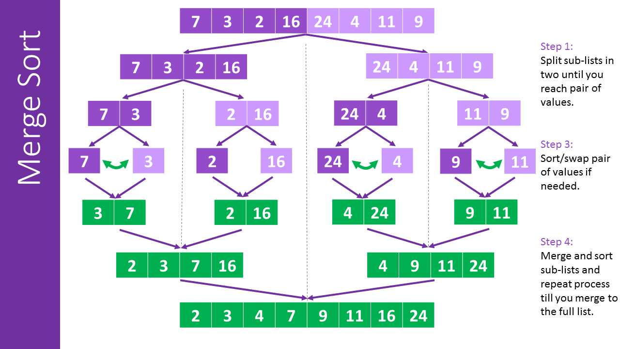
O(n*log(n)) - Merge Sort
Selection sort isn’t a good sorting algorithm when dealing with large lists. Merge sort is a divide-and-conquer algorithm and it’s much better than the quadratic time from Selection Sort.
Merging two sorted lists is linear in the length of the lists, so the time complexity of merge() is O(len(L)). The time complexity of merge_sort() is O(len(L)) multiplied by the number of levels of recursion. Since merge_sort() divides the list in half each time, the number of levels of recursion is O(log(len(L))). Therefore, the time complexity of merge_sort() is O(n*log(n)), where n is len(L).
def merge(left, right, compare):
    result = []
    i, j, = 0, 0
    while i < len(left) and j < len(right):
        if compare(left[i], right[j]):
            result.append(left[i])
            i += 1
        else:
            result.append(right[j])
            j += 1
    while i < len(left):
        result.append(left[i])
        i += 1
    while j < len(right):
        result.append(right[j])
        j += 1
    return result

def merge_sort(L, compare = lambda x, y: x < y):
    """Receive a list L and returns a new list with the same elements as L, but does not mutate L."""
    if len(L) < 2:
        return L
    else:
        mid = len(L)//2
        left = merge_sort(L[:mid], compare)
        right = merge_sort(L[mid:], compare)
        return merge(left, right, compare)
L = [9, 8, 8, 7, 6, 5, 4, 3, 2, 9, 0, 1]
sorted_list = merge_sort(L)
print("L =", L)
print("Sorted L = ", sorted_list)
print(sorted_list is L)
OUTPUT: L = [9, 8, 8, 7, 6, 5, 4, 3, 2, 9, 0, 1]
Sorted L = [0, 1, 2, 3, 4, 5, 6, 7, 8, 8, 9, 9]
False
The following image has a good visual explanation of what happens during the algorithm.
Resources
[1] - stackoverflow - Examples of Algorithms which has O(1), O(n log n) and O(log n) complexities
[2] - stackoverflow - Real-world example of exponential time complexity
[3] - “Introduction to Computation and Programming Using Python: With Application to Understanding Data”, John. V. Guttag, MIT Press.
[4] - Professor Eric Grimson - Simple Programs | Bisection Search