Sometimes it’s important to know how a program will behave when increasing the input size. Analyzing the running time of an algorithm is very important for problems with big data.

Here we’ll be talking about Big O notation as a way to predict the running time efficiency of a program as the input grows. In the next posts, I’ll be talking about each one of the important complexity classes.

Worst case scenario

Let’s suppose we have to search for an element n in a list L. We can analyze three scenarios of finding n in L:

def search(n, L):
    for num in L:
        if num is n:
            return True
    return False

• The best-case running time scenario is the minimum running time needed to find n inside L. If n is the first element inside the list, the number is found almost immediately. So, the best running time is independent of the size of L.

• The average-case or expected-case scenario is the average running time over all possible inputs.

• The worst-case running time scenario is the maximum running time over all the possible inputs. For searching an element n in L, the worst-case scenario is in the size of L, because the algorithm will have to look through every number in L once.

For analyzing algorithms, we will use Big O notation. Big O notation focus on the worst-case scenario, that provides an upper bound on the running time, that means it bounds a function only from above.

The search(n, L) function grows linearly so the complexity is in O(n).

What is Big O notation

Asymptotic notation is used as a way to visualize a relationship between the running time of an algorithm an the size of input. The question its come to answer is “how my program will behave when the input size is duplicated? triplicated?” and so on.

Big O notation is an asymptotic notation that will describe the complexity of an algorithm as the size of its inputs approaches infinity. It is a member of a family of notations collectively called Bachmann-Landau notation.

The main rules in describing the asymptotic complexity of an algorithm are:

• If the running time is the sum of multiple terms, only the one with the largest growth rate will matter to the analysis.

• If the remaining term is a product, drop any constants.

For the following function

def f(n):

    # Loop that takes constant time
    for i in range(10):
        print(i)

    # Loop that takes n time
    for i in range(n):
        print(i)

    # Loop that takes n**2 time
    for i in range(n):
        for j in range(n):
            print(i, j)

assuming that each line of code takes one unit of time to execute, the running time of this function is (10 + n + 2n²). The big O notation is in O(n²), because to asymptotic analysis, only the predominant term matters, because always n < n² and 100 < n² and the constant 2 is dropped off.

Important Complexity Classes

• O(1) - denotes constant running time
• O(log(n)) - denotes logarithmic running time
• O(n) - denotes linear running time
• O(n(log(n))) - denotes log-linear running time
• O(n^k) - denotes polynomial running time; k is a constant
• O(c^n) - denotes exponential running time; c is a constant

More at the top, better is the algorithmic complexity. Check the following graphic to see how each one of this functions behave as the input size grows.

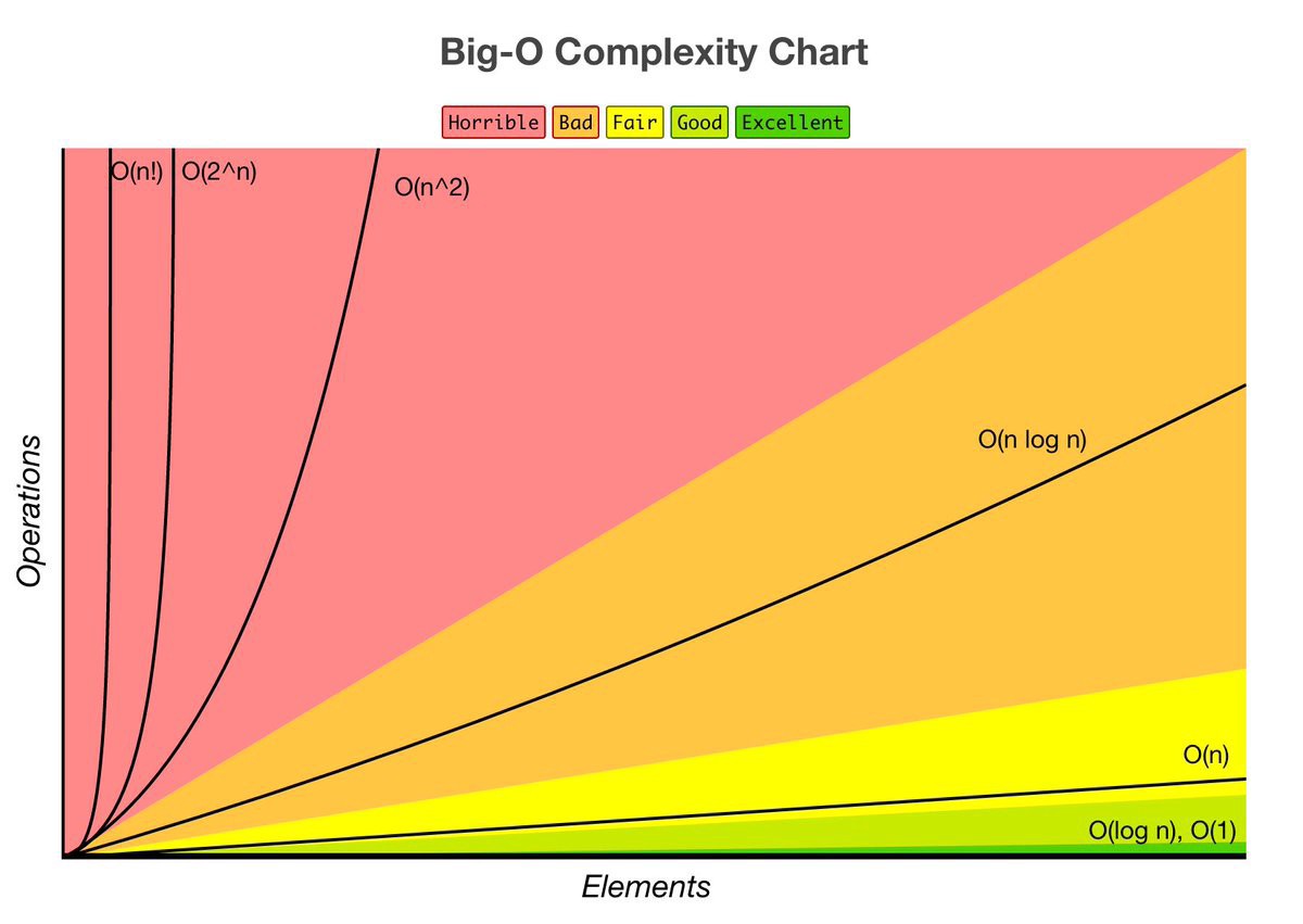Image from bigocheatsheet.com

Resources

This post was based on the amazing lectures of Professor Eric Grimsom, that I highly recommend:

• Lecture 10: Understanding Program Efficiency, Part 1
• Lecture 11: Understanding Program Efficiency, Part 2
• Lecture 12: Searching and Sorting

And in the (also amazing) book:

• “Introduction to Computation and Programming Using Python: With Application to Understanding Data”, John. V. Guttag, MIT Press.